Real GDP: The Flawed Metric at the Heart of Macroeconomics
May 1, 2019
Blair Fix, Jonathan Nitzan and Shimshon Bichler
The study of economic growth is central to macroeconomics. More than anything else, macroeconomists are concerned with finding policies that encourage growth. And by ‘growth’, they mean the growth of real GDP. This measure has become so central to macroeconomics that few economists question its validity. Our intention here is to do just that.
We argue that real GDP is a deeply flawed metric. It is presented as an objective measure of economic scale. But when we look under the surface, we find crippling subjectivity. Moreover, few economists seem to realize that real GDP is based on a non-existent quantum — utility. In light of these problems, it seems to us that much of macroeconomics needs to be rethought.
1. Calculating Real GDP
Macroeconomists entertain two related measures of GDP: nominal GDP, which is the total money value of goods and services produced in an economy in a given period (say a year); and real GDP, which is the total quantity of these same goods and services.
The challenge for macroeconomists is that the ‘quantity’ of goods and services — and therefore real GDP — cannot be aggregated directly. Since goods and services are qualitatively different, economists cannot sum their quantities in their natural units (try adding 10 lb of tomatoes to two laptops to five financial services). While each commodity bundle has its own quantity, these quantities are incommensurable.
Fortunately, there is a simple way around this difficulty — or so say the macroeconomists. To understand their solution, we need to backtrack a bit. Unlike real GDP, nominal GDP can be readily calculated in universal money terms. If the price of a commodity i is P_i and its quantity is Q_i, then its money value {Y_i = Q_i \times P_i}. Aggregating the money values across all n commodities produced in the economy gives us nominal GDP:
1. nominal GDP \displaystyle = \sum_{i=1}^n Y_i = \sum_{i=1}^n Q_i \times P_i
As Equation 1 makes clear, over time nominal GDP can grow or contract for two reasons: (1) because quantities change (through greater or lesser production), and (2) because prices change (via inflation or deflation). And here, say the macroeconomists, lies the solution: if we ‘purge’ nominal GDP from the effect of inflation and deflation, we end up with real GPD.
This purging is technically straightforward. Instead of multiplying each commodity by its current money price P_i (which changes from year to year), we multiply it by the price prevailing in a particular ‘base year’ Pb_i. In this calculation, prices are always the same, by definition. And since the only things that change now are the quantities being produced, we end up with real GDP denominated in base-year prices:
2. real GDP {\displaystyle = \sum_{i=1}^n Q_i \times Pb_i}
2. Which Base Year?
But there is a slight conceptual problem. It turns out that the growth of real GDP — ostensibly a single, objective quantity — is highly sensitive to our choice of base year.
To illustrate, consider a hypothetical economy that produces only two commodities: 1,000 lb of tomatoes and two laptops. Next, let’s choose 1990 as our base year and assume that tomatoes in that year cost $2/lb while a laptop costs $2,000. In this case, real GDP, denominated in 1990 dollars, would be $6,000 (=1,000 \times $2 + 2 \times $2,000). Now, skip to 1991 and imagine that, in that year, the economy grows by producing one additional laptop. This increase means that real GDP in 1991, denominated in 1990 prices, is $8,000 (=1,000 \times $2 + 3 \times $2,000). Compared to 1990, real GDP grew by 33.3 per cent .
So far so good. Now, instead of using 1990 as our base year, let’s use 1991. Production levels remain unchanged: 1,000 tomatoes and 2 laptops in 1990, and 1,000 tomatoes and 3 laptops in 1991. Base-year prices, though, are no longer the same: in 1991, our newly chosen base year, tomato prices double to $4/lb, while laptop prices are halved to $1,000. Under these new conditions, real GDP for 1990, this time denominated in 1991 dollars, is $6,000 (=1,000 \times $4 + 2 \times $1,000), while real GDP for 1991, also in 1991 dollars, is $7,000 (=1,000 \times $4 + 3 \times $1,000). Unlike before, in this example real growth is only 17 per cent .
In other words, real GDP is affected not only by the actual quantities being produced, but also by our choice of base year. And since there are numerous base years to choose from, the same real GDP can end up having many different magnitudes! [1]
3. Inherent, Irreducible Uncertainty
The base-year problem logically means that there is uncertainty in real GDP. Because relative commodity prices change from year to year, each base year will generate a different measure of real GDP. And since there is no way to determine which base-year measure is ‘correct’, the choice is always arbitrary. This arbitrariness leaves us with inherent, irreducible measurement uncertainty.
Here is the curious thing: economists do not report this uncertainty. Scientists know that measurement uncertainty must be reported. The uncertainty indicates the confidence in the measure. The larger the uncertainty, the less confident we are. If we do not report uncertainty, we are not telling the truth to other scientists. We make our measure appear certain when it is not. Although economists are aware of the base-year problem (it is taught to undergraduates), one will never find an official measure of the uncertainty in real GDP growth data. The government publishes only one measure of real GDP, with no reported uncertainty.
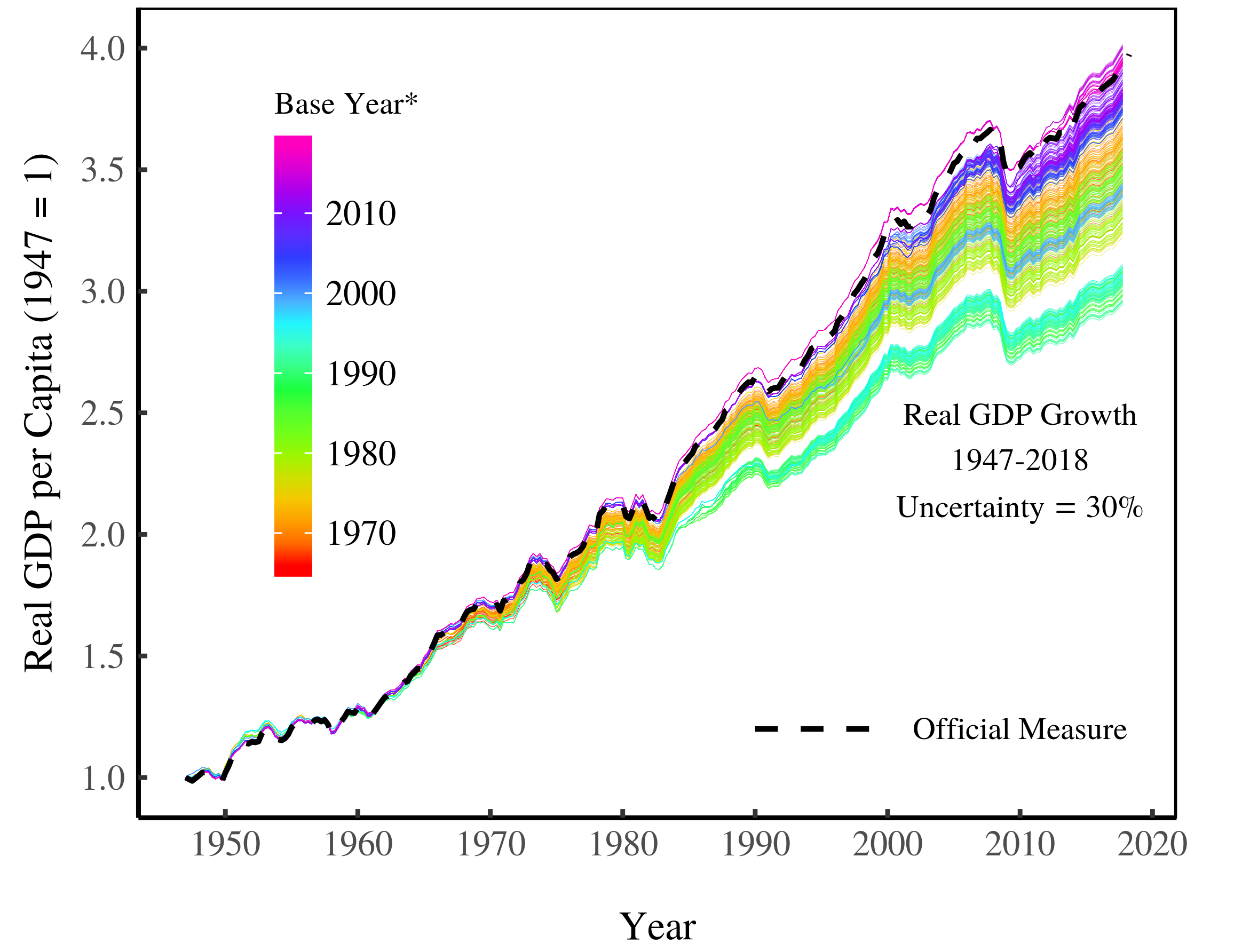
In a recent paper, Blair Fix (2019) estimates the uncertainty in real GDP resulting from the base-year problem. To reiterate, this uncertainty is caused by instability in relative prices. Over the long term, this instability is spectacular. Figure 1A shows the divergent price change of 10 selected commodities from the US Consumer Price Index. Figure 1B shows the price change of all CPI commodities. Figure 1C shows the resulting uncertainty in real GDP growth — about 30 per cent since 1947. [2]
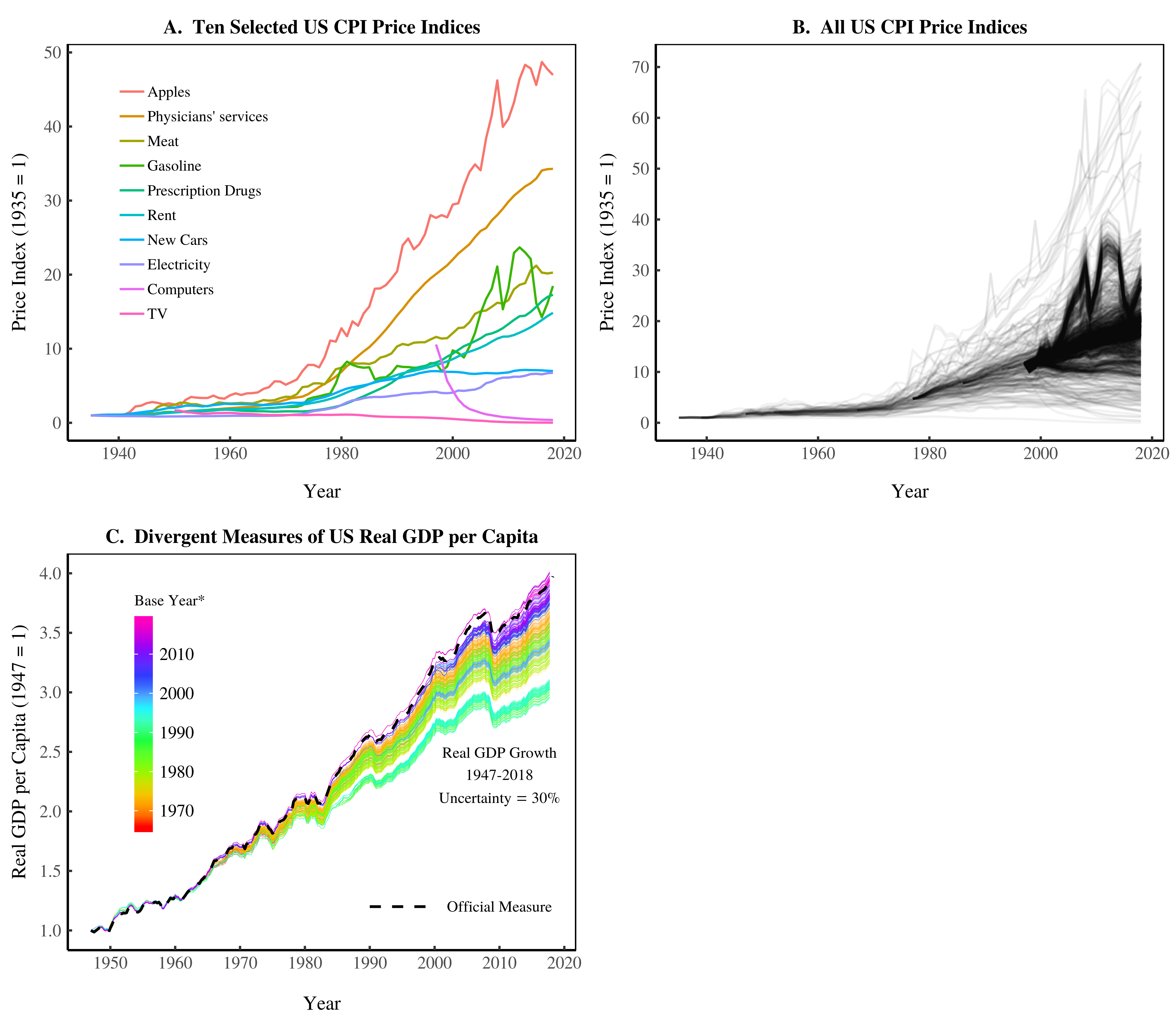 Figure 1: Divergent Price Change and Divergent Measures of Real GDP.
This figure was first published in Fix (2019). It shows how divergent changes in price affect the measurement of US real GDP. Panel A shows historical price changes in ten selected commodities tracked by the Bureau of Labor Statistics. Panel B shows divergent price change for all CPI commodities. Divergent price change means that the choice of base year has a strong effect on the measurement of real GDP growth, as shown in Panel C. For sources and methods, see the Appendix in Fix (2019).
Curiously, the official measure of real GDP is right at the upper range of this uncertainty. Is this a coincidence? Or have government statisticians simply chosen the method that yields the maximum growth (so as to appease their superiors)? This is an important question that, as far as we know, remains uninvestigated.
4. Chain-Weighting the Base-Year Problem
To reiterate, the base-year problem leads to uncertainty in the calculation of real GDP. But instead of openly reporting this uncertainty, government economists have devised a ‘fix’. Rather than using a single base year, they ‘chain’ together many adjacent base years. This is a bit like a moving average. They calculate the growth of real GDP between consecutive years, using the first year as the base, and then ‘chain’ together the resulting growth measures to calculate real GDP levels. This method claims to ‘fix’ or at least lessen the base-year problem. It doesn’t.
The appeal of chain-weighting, according to economists, is that it gets closer to their theoretical ideal. According to this ideal, the weight of each commodity in real GDP is provided by its ‘true’ or ‘natural’ price. When using a single base year, the implicit assumption is that relative prices in that base year are ‘true’ and therefore constitute the ‘correct’ weights (Equation 2). However, if the ‘correct’ weights change over time, and if these changes are mirrored in the movement of relative market prices, we can do better by changing the base year more often (every year) and chain-weight the results.
This argument is superficially convincing, but it falls apart on further inspection. Chaining together base years is better than using a fixed base year only if the ‘true’ weights indeed change over time, and only if ‘truth’ here is indeed revealed by relative market prices. Unfortunately, there is no way to ascertain either ‘if’. And as long as these two ‘ifs’ remain hanging — which might be forever — chain-linked measures must be deemed as arbitrary as their fixed-based cousins.
The only solution to the base-year problem would be if prices were stable. But since we cannot change history, this solution is unattainable. [3]
5. Unknowable Unknowns: Quality Change
And this is just the tip of the iceberg. Lurking underneath the base-year issue is a far bigger problem — the measurement of quality change. And unlike the base-year problem, the scope of the quality-change problem is difficult, if not impossible, to estimate quantitatively.
When measuring price change, economists attempt to adjust for changes in the quality of a commodity. An increase in the quality of a commodity is recorded as an increase the quantity of real GDP. So if computers get 10 times better, then computer output is recorded as increasing by a factor of 10.
And here arises the question: how do we measure quality change? Before diving into the specifics, we should recognize that there is little agreement on this topic. The governments of the world use different methods, and the result is wildly different measures of quality change.
Take computers. Figure 2 shows the different measures of computer quality change used by eight different OECD countries. Now, to a first approximation, computers are the same everywhere. So these different measures reveal nothing about the actual change in computer quality. They are just an artefact of the different methods being used. If we project these different quality-change measures over 30 years, the divergence is spectacular. Assuming no change in the underlying number of computers produced, we find a 1,000-fold disparity in the growth of computer output across the different countries. Clearly, we have a problem.
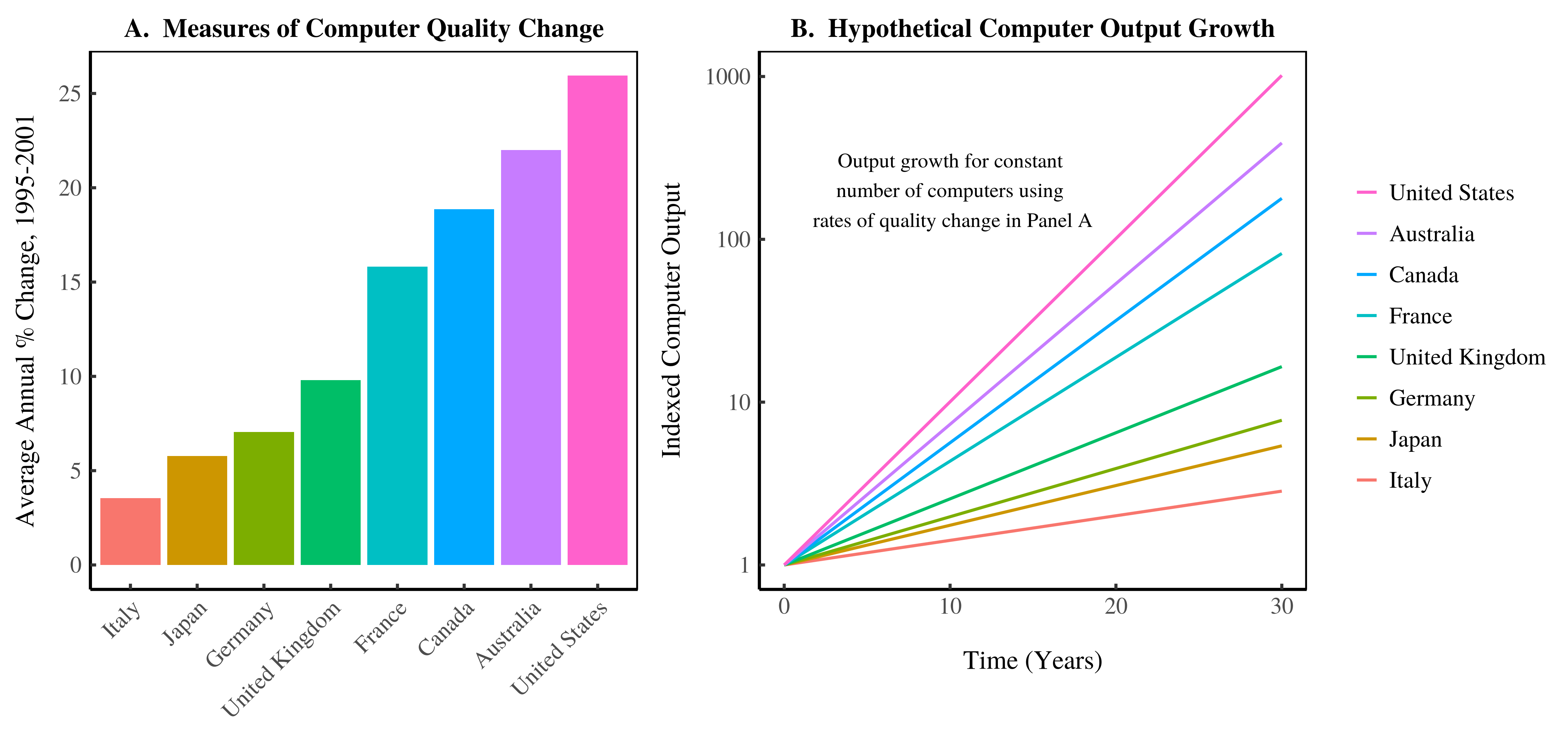
Figure 2: Divergent Measures of Computer Quality Change.
This figure was first published in Fix (2019). It illustrates the dispersion in national estimates of computer quality change. Panel A shows computer quality change estimates for eight OECD nations. Bars represent the average annual growth rate of computer quality between 1995 and 2001. Panel B shows how these quality-change measurements would affect the growth of computer ‘output’ over 30 years. Assuming the number of computers produced remains the same in each year, the different quality adjustments lead to divergent measures of computer output growth spanning three orders of magnitude
The problem is that measuring quality change requires numerous subjective decisions. There are so many such decisions, in fact, that it is virtually impossible to keep track of the ways that quality changes affect the measure of real GDP.
Natural scientists have the concept of ‘error propagation’. In each step of analysis, we have uncertainty in our measurement. To keep track of this uncertainty, we ‘propagate’ it through our calculation. If economists were serious scientists dealing with an objective reality, they would do the same with real GDP. Each time they made a subjective decision about how to measure quality change, they would keep track of the results that would have occurred if other choices had been made. This would give a possibility space for the range of possible measures of real GDP.
How large is this possibility space? We have no idea. In fact, since quality is partly subjective, this space might be undefinable (more on this below). But even if it can be defined, governments report only one measure of quality change. It is thus virtually impossible to know how alternative ways of measuring quality change would affect the measure of real GDP growth. This is an ‘unknowable unknown’. At present, there is no way to estimate the uncertainty in real GDP that results from different ways of measuring quality change. And not only can we not answer this question, but most macroeconomists are not even interested in asking it. To ask the question is to admit the arbitrary nature of real GDP.
6. The Unasked Question: What is the Unit of Real GDP?
Most economists believe that ‘constant dollars’ — i.e. dollars expressed in fixed prices of a given year — are the unit of real GDP. For instance, the Federal Reserve Bank of St. Louis reports that real GDP has units of ‘Chained 2012 Dollars’. Unfortunately, this belief is false — or, worse still, meaningless. It is logically untenable when we reflect on the methods that go into measuring real GDP.
As soon as we start ‘adjusting’ for quality change, we are no longer using prices as the unit of analysis. Instead, we are appealing to some other unit — the unit of quality that is hidden in the commodity. What is this unit? It is utility — the quantity of pleasure that consumers derived from a commodity. Here is the US Bureau of Labor Statistics describing how ‘hedonic’ adjustments appeal to ‘utility’ to measure quality change:
In price index methodology, hedonic quality adjustment has come to mean the practice of decomposing an item into its constituent characteristics, obtaining estimates of the value of the utility derived from each characteristic, and using those value estimates to adjust prices when the quality of a good changes. (Bureau of Labor Statistics 2010)
The problem is that this utilitarian approach is built on foundations of sand. Utility, even if it were commensurable across individuals, is unobservable directly. But economists are not deterred. They hypothesize that prices reveal the utility of a commodity. They then use prices to estimate the utility embodied in each characteristic of the commodity. This method allows them, or so they think, to measure quality change.
Unfortunately, the whole operation is circular. And when we look at the logic closely, it is indefensible. Prices are taken to reveal the utility of a commodity. But having made this assumption, we then find that prices change through time. This means that nominal prices cannot be trusted to reveal utility. So we have to ‘correct’ for price change to measure the ‘true’ change in utility. But we make this correction by appealing to prices — the very unit we just rejected. The logic is torturous when stated clearly.
In reality, economists never get close to measuring utility. Instead, their hedonic quality adjustment is an arbitrary algorithm for calculating quality change. It is based on a host of subjective decisions. These include the choice of the relevant characteristics of the commodity, the choice of functional form of the hedonic regression used to weigh these characteristics and the choice of the cross-section method. Different assumptions will yield different measures of quality change. And there is no way to know which measure, if any, is ‘correct’.
As a PhD student, Jonathan Nitzan wrote a paper pointing out these difficulties in quality-change measurement (Nitzan 1989). But he found that the paper was unpublishable. He was scolded by reviewers. ‘These problems have been solved’, they said. Unfortunately, the supposed ‘solutions’ remain unknown to us, some 30 years later. In fact, we think that the problems are unsolvable. Economists assume that utility is the unit of quality. But this unit is unobservable — or put more strongly, it is non-existent (Nitzan and Bichler 2009).
To summarize, whether openly or tacitly, the methods used for quality-change adjustment take the true unit of real GDP to be utility. To justify measuring aggregate utility, economists need a host of assumptions. These are:
- All consumers must be identical. This identity ascertains that utilities are commensurable and substitutable, and that the quantities of commodities, measured in utility, are independent of whoever happens to own them.
- Consumer preferences must be independent of income, so that a redistribution of income from poorer to richer consumers, or vice versa, will not alter the utility generated by a given array of goods and services.
- Preferences must remain temporally fixed to ascertain that, over time, a given array of goods and services will yield the same measure of ‘real GDP’.
- All markets must be in a perfectly competitive equilibrium to ascertain that prices reflect the underlying utilities; alternatively, economists must know the ‘correct’ prices that would have prevailed had markets been in a perfectly competitive equilibrium.
Since assumptions 1–4 are never satisfied, the resulting measures of ‘real GDP’ are meaningless. In our view, the correct acronym for ‘real GDP’ should be AWUGDU — pronounced ‘a-woogdoo’. It stands for ‘Arbitrarily Weighted Unquantifiable Gross Domestic Utility’.
7. Solutions: Differential Measures for Prices and Biophysical Measures for Scale
If real GDP is largely meaningless, as we have argued, the result is a conceptual void that fundamentally undermines the field of macroeconomics. It means there is no single measure of economic output on which to build a theory of economic growth. Consequently, much of macroeconomics must be questioned.
If we discard real GDP, then what are the alternatives?
We propose two different approaches. First, if we are interested in prices, then there is no need to use inflation-adjusted metrics. We can simply compare the price of one commodity to the price of another. We call this a ‘differential’ measure. Nitzan and Bichler (2009) have proposed a theory of capitalism that appeals only to differential measures. They call it capital as power, or CasP for short. The idea is that, as capitalism advances and spreads, the relative prices of owned commodities reflect the power structure of society. When we study differential prices such as those of Amazon’s stock relative to Apple’s, we are implicitly studying the relative power of the owners of these two companies.
Regardless of whether one accepts this ‘capital as power’ hypothesis, differential prices can be studied objectively. But we must be sure that, whenever possible, we use actual nominal prices, not the price indexes reported by statistical agencies (since these contain subjective quality-change adjustments).
Second, if we are interested in the overall scale of the economy we can use biophysical measures. Fix (2015b, 2015a) has argued that energy use is an important measure of economic scale. Keen, Ayres and Standish (2019) have recently reiterated this idea. The laws of thermodynamics dictate that energy is essential for sustaining complex systems. Its necessity makes it a prime candidate for measuring economic scale.
Energy use can help us scientifically define the boundaries of production, as well as to assess the impact of that production on the biosphere. Note, however, that we do not equate more energy use with a better quality of life. More energy use is simply more energy use. To measure the quality of life — and human wellbeing more generally — we need a new accounting system altogether. This system must be based not on neoclassical notions of perfect competition and individual utility, but on a democratic articulation of what constitutes the ‘good life’ and a ‘good society’ within our broader biosphere.
Endnotes
[1] For visual illustrations of the base-year effect, see Nitzan and Bichler (2009: Ch. 8), Bichler and Nitzan (2015) and Fix (2019: Section 2.2).
[2] Note that this estimated range of uncertainty assumes that at least one of the years since 1947 was a ‘correct’ base year. However, if that assumption is false — in other words, if the ‘correct’ set of relative prices was never mirrored in prevailing market prices — the range of possible real GDP measures can be much wider. Worse still, if we reject the very notion that there is a ‘correct’ set of relative prices to start with, estimating the uncertainty range becomes impossible if not totally meaningless. The best we can do, then, is speak of a ‘possibility space’ for real GDP, defined by the range of subjective measurement choices.
[3] One of us (Fix) recently engaged in a lengthy debate with an (anonymous) economist who defended the practice of chain-weighting GDP. The exchange can be found on the capitalaspower.com forum.
References
Bichler, Shimshon, and Jonathan Nitzan. 2015. Capital Accumulation: Fiction and Reality. Real-World Economics Review (72, September 30): 47-78.
Bureau of Labor Statistics. 2010. Frequently Asked Questions about Hedonic Quality Adjustment in the CPI. Retrived June 24, 2013, from https://www.bls.gov/cpi/quality-adjustment/questions-and-answers.htm.
Fix, Blair. 2015a. Putting Power Back Into Growth Theory. Review of Capital as Power 2 (1): 1-37.
Fix, Blair. 2015b. Rethinking Economic Growth Theory from a Biophysical Perspective. New York: Springer.
Fix, Blair. 2019. The Aggregation Problem: Implications for Ecological and Biophysical Economics. BioPhysical Economics and Resource Quality 4 (1): 1-15. </p?
Keen, Steve, R. U. Ayres, and Russell Standish. 2019. A Note on the Role of Energy in Production. Ecological Economics (157): 40-46.
Nitzan, Jonathan. 1989. Price and Quantity Measurements: Theoretical Biases in Empirical Procedures. Working Paper 14/1989, Department of Economics, McGill University, Montreal, pp. 1-24.
Nitzan, Jonathan, and Shimshon Bichler. 2009. Capital as Power. A Study of Order and Creorder. RIPE Series in Global Political Economy. New York and London: Routledge.